Go big or go OOM: the art of scaling vLLM

TL;DR

Sharing LLM-as-a-Judge (JLM) deployments across multiple concurrent training jobs can reduce GPU underutilization, but makes the deployment vulnerable to buckling under load. We mitigated this by applying a two-pronged approach: optimizing single-node performance and scaling multi-node deployment, arriving at a strategy applicable to any high-throughput inference deployment facing variable load.

The challenge: multi-node LLM deployments that don’t buckle under load 

During the final training stage of our Jamba model family, we introduced a custom implementation of online-RL (GRPO). Online RL training requires a reward function that steers model behavior in the right direction. For verifiable tasks such as math, the reward can be easily defined with a deterministic function. However, freeform tasks (e.g., question-answering and instruction-following) require more complex, model-based rewards – which we implement using LLMs-as-a-Judge (JLMs).

In a classic online RL setting, JLMs are used only during the reward phase and sit idle for the rest of each GRPO training step, leading to GPU underutilization. One way to mitigate this is a fully async approach, which maximizes GPU utilization per training job but introduces other complexities and constraints. Another solution is to share JLM deployments across multiple training jobs – when one job is busy with a policy update, others can use the otherwise-idle JLMs.

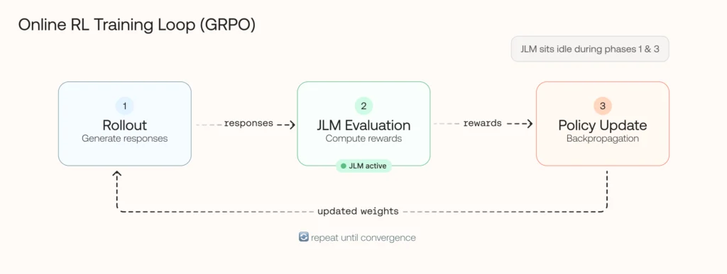
This improved GPU utilization, but also exposed the JLMs to unpredictable bursts of traffic from multiple sources. We needed to make the JLM deployments robust enough to handle multiple concurrent training jobs without buckling under load. In this post, we share the process we went through and the lessons we learned.

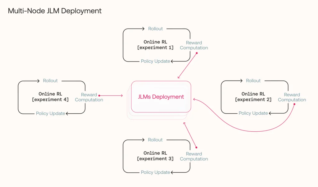
While our use case focused on JLM serving for GRPO training, these principles apply to any high-throughput vLLM deployment facing variable load, whether you’re serving chat applications with traffic spikes, running batch inference, or supporting ML training pipelines like ours.

Let’s dive in.

The two-angle approach: the key to optimizing multi-node LLM deployments

Like many classic system architecture challenges, we chose to tackle this problem by introducing optimizations from two angles: the vertical (single-node performance) and the horizontal (multi-node scaling).

The vertical angle: optimizing single-node performance

Since we use vLLM as the inference framework for our JLMs, we started by examining vLLM’s configuration. The vLLM engine exposes numerous arguments controlling its execution, from batching strategy and batch size to memory allocation and utilization. By tuning these parameters for our specific sequence lengths, load patterns, model architecture, and hardware, we could significantly improve performance and GPU utilization.

We used OpenShift’s Auto-Tune vLLM, which leverages GuideLLM for benchmarking and Optuna for multi-objective hyperparameter optimization.

Step 1: Analyzing our workload

Before running Auto-Tune, we needed to make decisions about several key parameters:

1. Sequence length distribution: Minimum, maximum, and average input/output lengths. These numbers guide how synthetic test data is generated and distributed to match real traffic patterns.
2. Traffic pattern: Are requests arriving in bursts or as a constant stream? This affects vLLM’s batching configuration – for instance --max-num-seqs. For bursty traffic (like ours), vLLM needs a high value to absorb large request spikes into a single batch. For constant-rate traffic, a lower value can reduce individual request latency.
3. Optimization target: Are we optimizing for throughput or latency? In other words, do we care more about individual request duration or total batch processing time?

Since our JLM’s clients are our own training runs, we could answer these questions by examining our evaluation patterns:

Step 2: Configuring the parameters for the optimization run

With our workload characterized, we configured the optimization run. We used Auto-Tune vLLM with NSGA-II strategy, a multi-objective genetic algorithm, to explore the parameter space and find Pareto-optimal configurations.

Search space

This is the search space we defined for the algorithm – vLLM engine arguments we wanted to optimize and the range of values to be tested for each:

Benchmark configuration

Each candidate configuration was tested with synthetic traffic matching our workload:

• 2K input tokens (varying up to 8K)
• 100–1K output tokens
• Rate of 2k concurrent requests
• 5-minute timeout per trial

Optimization objectives

We defined the optimization metrics according to which each candidate configuration should be evaluated:

• Output tokens/second (maximize)
• Requests/second (maximize)
• Request latency (minimize)
• Time-to-first-token (minimize)
• Inter-token latency (TPOT) (minimize)

Step 3: Running the trials

The optimization ran 300 trials, of which 125 completed successfully. Some configurations encountered OOM errors or timed out – but this is expected and handled gracefully by the framework.

Step 4: Picking the winning configuration

Since we optimized for five metrics simultaneously, we were left with 24 Pareto-optimal configurations representing different tradeoffs between the list we outlined above. Since our goal was maximizing throughput, because we needed the complete reward computation to finish as quickly as possible before proceeding to the policy update phase, we selected the configuration with the highest token throughput.

This is the resulting vLLM config:

Model: 32B dense attention model
Hardware: H100 SXM 80GB

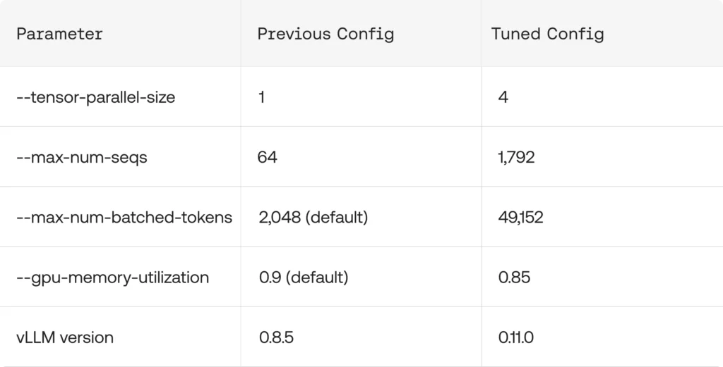
Looking at the results, you might think – of course the tuned config produced better throughput than the old one – it used 4 times more GPU resources!

The answer to that is rooted in the way we evaluate the configurations:

When comparing configurations, we evaluate throughput at the deployment level. Given a fixed GPU budget, how should we distribute them across vLLM processes for best performance?

The equation is:

num_instances = total_gpus / tensor_parallel_size 

total_throughput = num_instances × throughput_per_instance

Since we tested tp ∈ {1, 2, 4, 8}, we can normalize to 8 total GPUs for comparison. The fact that tp=4 produced the optimal scores means that 2× 4-GPU instances outperformed:

• 8× 1-GPU instances
• 4× 2-GPU instances
• 1× 8-GPU instance

Why tp=4? We can’t say definitively, but we suspect it hits a sweet spot for our workload: with tp=1, each instance has limited memory for KV cache, restricting how many concurrent requests it can handle – problematic for our bursty traffic pattern. Moving to tp=4 pools memory across 4 GPUs, allowing significantly more concurrent sequences. But tp=8 likely suffers from diminishing returns: the cross-GPU communication overhead grows while the additional KV cache capacity provides less marginal benefit. For our specific use case, tp=4 appears to be the right trade-off.

Step 5: Measuring the gains

Before comparing the performance of the old configuration against the tuned one, we needed to isolate the impact of the vLLM version upgrade on the results. To do this, we ran three separate tests using GuideLLM:

• The old config on the old vLLM
• The old config on the new vLLM
• The tuned config on the new vLLM

We used the following test commands:

Old configuration (rate and max-requests reflect load distributed across 4× 1-GPU instances):

guidellm benchmark \
  --target "http://localhost:8000" \
  --profile throughput \
  --rate 25 \
  --max-requests 500 \
  --data "prompt_tokens=2000,output_tokens=500"

Tuned configuration (single 4-GPU instance):

guidellm benchmark \
  --target "http://localhost:8000" \
  --profile throughput \
  --rate 100 \
  --max-requests 2000 \
  --data "prompt_tokens=2000,output_tokens=500"

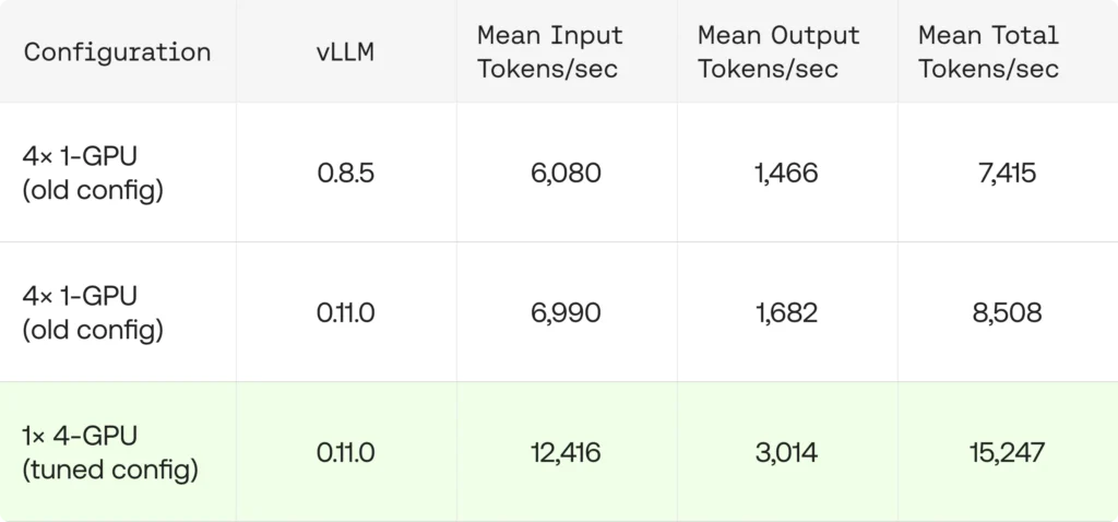
With that isolation established, we could finally take a look at our benchmarks to measure the amount of improvement. Looking at our primary metric of throughput, it’s clear that the last test – tuned config on the new vLLM – performed best.

Throughput results (4 GPUs total)

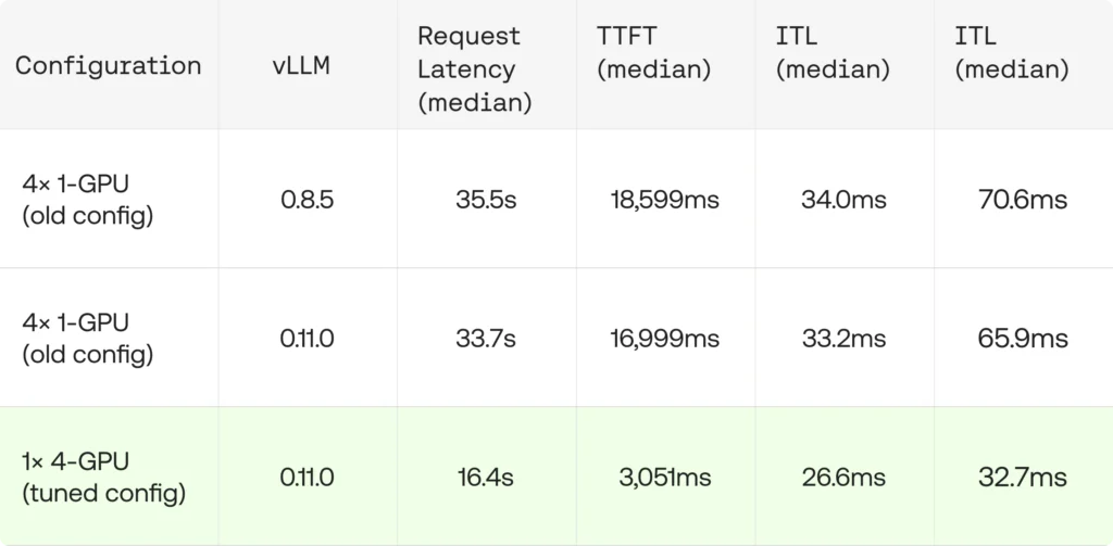
If we also take a look at latency, another key metric, we see that, once again, the tuned config on the new vLLM version performed best.

Latency results

So, what could be behind this improvement?

Upgrading vLLM from v0.8.5 to v0.11.0 with identical configuration gave us modest gains: ~15% better throughput and ~5% lower latency. Respectable, but we could do much better.

The real wins came from configuration tuning. Returning again to our core metrics, let’s compare the performance of the old config versus the tuned config, both running on vLLM v0.11.0:

Combined, we achieved roughly 2× throughput and 2× lower latency from the same 4 GPUs.

The lesson: Upgrading vLLM versions is worthwhile, but it won’t rescue a misconfigured deployment. For our bursty, throughput-heavy workload, the old vLLM settings were leaving substantial performance on the table.

The horizontal angle: scaling multi-node deployment

While the vertical optimizations gave us significant per-instance improvements, they weren’t enough to handle the unpredictable load of multiple concurrent training jobs. To solve that, we took a horizontal approach: dynamically scaling the JLMs deployment.

Step 1: Defining an autoscaling metric

On its surface, dynamically scaling requires defining an autoscaling metric for our vLLM instances. But choosing the right one is not straightforward.

Let’s examine some typical autoscaling indicators and why they fail for LLM inference:

• Resource utilization:
  • GPU utilization: A fully utilized GPU is exactly what we’re aiming for with proper configuration. 100% GPU utilization isn’t a sign of overload – it’s a sign of efficiency. Scaling up based on GPU utilization would trigger constantly, even when the system is handling load comfortably.
  • Memory utilization: vRAM used for KV cache fluctuates as requests complete and new ones arrive – high utilization might indicate healthy batching rather than overload. Host memory, used primarily for the request queue, is typically abundant and won’t be the bottleneck.
• Throughput metrics:
  • Metrics like input tokens/sec or output tokens/sec plateau once the instance reaches saturation. Beyond that point, throughput stays steady while new requests pile up in the queue. Throughput alone can’t distinguish between “handling load well” and “drowning in backlog.”

So perhaps we should look at the backlog itself?

Let’s recap quickly how vLLM handles incoming requests:

1. Incoming requests are queued before being scheduled for processing.
2. The continuous batching mechanism schedules requests from the queue up to the limits defined by –max-num-batched-tokens and –max-num-seqs.
3. Remaining requests wait in the queue (in CPU memory) until GPU space becomes available.

With that in mind, we can see that a good indication of an overloaded instance might be what the client actually experiences: requests taking longer and longer to get a response because the queue keeps growing. We can describe this as client-perceived latency.

vLLM exposes two Prometheus metrics that capture this:

• vllm:num_requests_waiting: The number of requests currently queued, waiting to be scheduled.
• vllm:request_queue_time_seconds: How long requests spend waiting in the queue before processing begins.

Both reflect the same underlying signal: when the instance can’t keep up with incoming load, the queue grows and wait times increase. While these metrics aren’t perfect because they’re influenced by sequence length, they still provide a good indication of client-perceived latency.

We chose queue size over queue time for simplicity: it’s a direct count that’s easy to reason about and tune.

Step 2: Implementing our HPA configuration

For our Horizontal Pod Autoscaler (HPA), we chose to scale based on average queue size across all pods in the deployment. When the mean vllm:num_requests_waiting crosses a defined threshold, Kubernetes spins up additional instances.

For minimum replicas, we set a number high enough to handle sudden bursts while new instances spin up.

deployment:
  autoscaling:
    minReplicas: 2
    maxReplicas: 10
    metrics:
      metric:
        name: vllm:num_requests_waiting
      target:
        value: 1000

Step 3: Finding the right threshold

The threshold of 1,000 pending requests per pod was determined empirically – it corresponds roughly to the point where queue wait times start impacting our training job timeouts. With our tuned configuration handling bursts of ~4K requests efficiently, an average queue of 1,000 indicates we’re approaching capacity and should scale out.

A few practical tips from our experience:

• Scale-up decisions are fast, but instance startup is slow: vLLM instances take significant time to initialize – loading model weights onto GPUs, profiling, and compiling CUDA kernels/graphs. In our case, a new JLM instance takes approximately 3 minutes to become ready. This means your threshold should be “forgiving” enough to tolerate queuing while new instances spin up. A threshold that’s too aggressive will trigger scale-up too late, when requests are already timing out.
• Scale-down should be conservative: We configured a 15-minute stabilization window for scale-down to avoid thrashing. You don’t want to spin down an instance only to need it again minutes later, paying the startup cost repeatedly.
• Tune client-side timeouts and retries (if possible): Set request timeouts that account for queuing during scale-up – failing too fast just sends requests to the back of another queue. Use exponential backoff between retries to avoid piling onto an already-stressed system.

Recap: key recommendations

After deploying these changes and a few rounds of tweaking, our JLM deployments handled multiple simultaneous training jobs smoothly.

Here’s a summary of what we learned:

Vertical optimization

1. Know your workload: Before tuning, characterize your traffic – max and average sequence lengths, burst patterns, and whether you’re optimizing for throughput or latency. This knowledge drives every configuration decision.
2. Use automated tuning: Tools like Auto-Tune vLLM can explore the configuration space systematically. Manual tuning is tedious and often misses non-obvious optima (like our tp=4 finding).
3. Revisit your configuration: Our previous --max-num-seqs (64) and --max-num-batched-tokens (2K, the default) were far too conservative for our workload. Tuning these to 1,792 and 49K respectively – combined with moving to tp=4 – unlocked 2× throughput and 2× lower latency from the same GPU budget.
4. Question your assumptions about tensor parallelism: A model fitting on one GPU doesn’t mean tp=1 is optimal. Test different configurations – the right balance between KV cache capacity and communication overhead depends on your workload.
5. Isolate your variables: When benchmarking, separate the impact of version upgrades from configuration changes. In our case, vLLM 0.8.5 → 0.11.0 gave ~15% improvement, but config tuning gave ~1.8× on top of that.

Horizontal scaling

1. Choose the right autoscaling metric: queue-based metrics like vllm:num_requests_waiting or vllm:request_queue_time_seconds that reflect client-perceived load can be a good indication of an overloaded instance.
2. Account for slow startup: vLLM instances take minutes to initialize. Set autoscaling thresholds high enough to tolerate queuing while new instances spin up.
3. Be conservative with scale-down: Use a long stabilization window to avoid thrashing and repeatedly paying the startup cost.
4. Align client timeouts with scaling delays: Account for scale-up delays; use exponential backoff to avoid amplifying load.